[Direct link to full PDF of this article]

Abstract: This document details the methodology for building, selecting, and filtering neutron and gamma-ray event cones for imaging in the context of the detector system composed of long-form-factor organic plastic scintillators developed in the NOVO project and as utilized in the ng-imager Python toolkit for neutron and gamma-ray imaging. A summary of the simple back projection method implemented is provided too. This work employs PHITS simulations of a simple six-bar detector array, providing data free of resolution effects and accompanied by extra “Monte Carlo truth” information to benchmark reconstruction method results against.

An experimental data pipeline, such as in the NOVO project, can be generally divided into five distinct main stages, requiring analysis procedures to progress from one stage to the next:

1. Raw detector data (integrated charges, timestamps, waveforms)

2. Physical quantities derived (energy deposited, interaction position, times)

3. Coincident events (physical quantities from double neutron / triple gamma-ray interaction coincidences, fulfilling various criteria)

4. Event cones (vertex, direction, half-angle)

5. Imaging (projection of event cones onto an imaging plane)

This work outlines the procedure for constructing neutron and gamma-ray event cones provided derived physical quantities from coincident events. Each particle contains some unique challenges in this regard. For neutrons, this includes determining the reaction’s nature (elastic scattering, inelastic scattering, or other nonelastic) and target (proton or carbon nucleus). For gamma rays, this includes determining the correct sequencing of the three reactions in coincidence to yield the most probable valid event cone. A condensed outline of the analytically-solved simple back projection imaging implementation used in ng-imager in “scan” mode is also provided.

Simulation setup

The simulations were conducted in PHITS (v3.29) [1] and set up as follows. Six parallel plastic scintillator bars of dimensions 12$\times$12$\times$140 mm$^3$ were arranged in a $3\times2$ pattern with a center-to-center spacing of 60 mm (48 mm gap width) to account for some real-world clearance for mounting hardware. The simulated design is pictured in Figure 1.

Figure 1. Simulated plastic scintillator array

In all neutron simulations, the source was an isotropic, 14.1 MeV monoenergetic neutron source placed 100 cm from the front face of the detector array and in line with its center. From the perspective of Fig. 1, the neutrons enter the picture from the lower left to then strike the array. While 100 million histories were simulated, the source was modeled as a cone with angle $\theta=5.5^\circ$ pointed toward the array, allowing simulation of only neutrons bound for the array. Owing to the cone’s 0.0289 sr solid angle, this was the equivalent of simulating 43.4 billion ($4.344\times10^{10}$) deuterium-tritium (DT) fusion events.

Provided the array is placed far enough from the source such that this source-to-array cone is only a few degrees wide, this monoenergetic assumption is valid. Likewise, a DT source is close enough to being completely isotropic for this assumption to hold as well.

Gamma-ray simulations employed a 2 MeV monoenergenic gamma-ray source otherwise identical to the neutron source described above. 1 billion histories (or an effective 434 billion emissions, corrected for solid angle) were simulated.

In a list mode fashion, neutron and gamma-ray interactions were recorded to “dump” files, and in post multiple scattering events were constructed, sequenced, and put into a new list for further tallying and analysis. Furthermore, neutron simulations included two tallies for interactions in the bars: one of only elastic scattering reactions and one for all nuclear reactions (including elastic scattering).

For the sake of events considered valid for imaging, only neutron double coincidences where each scatter deposited at least 500 keV were considered. This threshold was set to 100 keV for each of the three gamma-ray interactions.

Nuclear data libraries (JENDL-4.0) were employed for transport of neutrons $<20$ MeV instead of models (nucdata=1), and the event generator mode was enabled (e-mode=2) for accurate event-wise reaction data.

Cone construction and selection

Ultimately, each cone is defined by a vertex coordinate $O=(x_O,y_O,z_O)$ with an axis/direction vector $\hat{D}=\langle u,v,w \rangle$ and interior half-angle $\theta$. These are derived from the following physical quantities extracted from experimental data (and emulated in simulation):

• For neutron events:

  • 1^st scatter location $X_1=(x_1,y_1,z_1)$, time $t_1$, and energy deposited $E_{\mathrm{dep},1}$

  • 2^nd scatter location $X_2=(x_2,y_2,z_2)$ and time $t_2$

• For gamma-ray events:

  • 1^st scatter location $X_1=(x_1,y_1,z_1)$ and energy deposited $E_{\mathrm{dep},1}$

  • 2^nd scatter location $X_2=(x_2,y_2,z_2)$ and energy deposited $E_{\mathrm{dep},2}$

  • 3^rd scatter location $X_3=(x_3,y_3,z_3)$ (and energy deposited $E_{\mathrm{dep},3}$)

The process of creating event cones from this experimental/simulated data is referred to here as “cone construction.” For both neutrons and gamma rays, the vertex coordinate $O$ is the location of the first scatter, the direction vector $\hat{D}$ is the unit vector pointing from the second scatter to the first scatter, and the cone half-angle $\theta$ is the scattering angle of the first collision. The $\theta$ calculation differs for neutrons and gamma rays.

Neutron cone half-angle $\mathbf{\theta}$

For neutrons scattering elastically, the scattering angle in the center-of-mass (CoM) reference frame $\theta_{\mathrm{n,CoM}}$ is defined, with recoil nucleus energy $E_{\mathrm{recoil}}$, incident neutron energy $E_\mathrm{n}$, and ratio of the recoil nucleus’s mass to the neutron mass $A$ (Equation (1)), as [2]:

\begin{equation} A = \frac{m_\mathrm{recoil}}{m_\mathrm{n}} \label{atomicmass} \end{equation}

\begin{equation} \theta_{\mathrm{n,CoM}} = \arccos\left( 1 - \left( \frac{E_\mathrm{recoil}}{E_\mathrm{n}} \cdot \frac{(1+A)^2}{2A} \right) \right) \label{theta_CoM} \end{equation}

Experimentally, $E_\mathrm{recoil}$ is taken to be the energy deposited in the first scattering reaction $E_{\mathrm{dep},1}$. The scattered neutron’s energy $E_\mathrm{n}^\prime$ is determined with its time-of-flight (Equation (4)) and flight distance $s_\mathrm{n}$ (Cartesian distance between $X_1$ and $X_2$, Equation (5)) relativistically, with speed of light $c$, as:

\begin{equation} E_\mathrm{recoil} = E_{\mathrm{dep},1} \label{neutron_Erecoil} \end{equation}

\begin{equation} t_\mathrm{n,ToF} = t_2 - t_1 \label{neutron_tof} \end{equation}

\begin{equation} s_\mathrm{n} = \left| \vec{X_1X_2} \right| = \sqrt{ (x_1-x_2)^2 + (y_1-y_2)^2 + (z_1-z_2)^2 } \label{neutron_flightpath} \end{equation}

\begin{equation} v_\mathrm{n} = \frac{s_\mathrm{n}}{t_\mathrm{n,ToF}} \label{neutron_velocity} \end{equation}

\begin{equation} E_\mathrm{n}^\prime = \left( \sqrt{\frac{1}{1-(v_\mathrm{n}/c)^2}} - 1 \right) m_\mathrm{n}c^2 \label{neutron_KE} \end{equation}

For completeness’s sake, this would be calculated classically (non-relativistically) as shown in Equation (8). As shown in Figure 2, in the neutron energies relevant to proton therapy, the classical approach to calculating $E_\mathrm{n}$ deviates quite notably from the relativistic approach.

\begin{equation} E_\mathrm{n,\,non\text{-}relativistic}^\prime = \frac{1}{2}m_\mathrm{n}v_\mathrm{n}^2 \label{neutron_KE_classic} \end{equation}

Figure 2. What classical mechanics would predict a neutron’s kinetic energy to be at each true kinetic energy (as calculated relativistically using the same neutron velocity).

The incident neutron energy $E_\mathrm{n}$ is simply the sum of the scattered neutron energy $E_\mathrm{n}^\prime$ and the energy of the recoil product $E_\mathrm{recoil}$ (Equation (9)). Note that this assumption fails when the recoil product does not deposit all of its energy in the detection volume (and also fails when the reaction is nonelastic).

\begin{equation} E_\mathrm{n} = E_\mathrm{n}^\prime + E_\mathrm{recoil} \label{neutron_incident_KE} \end{equation}

The neutron scattering angle in the lab frame $\theta_{\mathrm{n,lab}}$ is found from $\theta_{\mathrm{n,CoM}}$ with:

\begin{equation} \theta_{\mathrm{n,lab}} = \arctan\left( \frac{\sin(\theta_{\mathrm{n,CoM}})} {\cos(\theta_{\mathrm{n,CoM}}) + (1/A)} \right) \label{theta_lab} \end{equation}

Strictly speaking, the $\mathop{\mathrm{atan2}}$ function, rather than $\arctan$, is used here as the desired output angle should range from 0 to $\pi$, not $-\pi/2$ to $\pi/2$. To avoid this, $\theta_{\mathrm{n,lab}}$ may also be equivalently expressed as [3]:

\begin{equation} \theta_{\mathrm{n,lab}} = \arccos\left( \frac{1 + A\cos(\theta_{\mathrm{n,CoM}})} {\sqrt{A^2 + 2A\cos(\theta_{\mathrm{n,CoM}}) + 1}} \right) \label{theta_lab_v2} \end{equation}

For the ease of discussion, when mentioning the neutron cone half-angle $\theta$ with no subscript, it is in reference to the lab frame $\theta_{\mathrm{n,lab}}$.

Gamma-ray cone half-angle $\mathbf{\theta}$

For a gamma ray undergoing solely Compton scattering in its first two interactions, the scattering angle of the first collision $\theta_{\gamma,1}$ can be found via Compton scattering kinematics [4]. First, the scattering angle of the second interaction $\theta_{\gamma,2}$ is calculated from the vectors $\overrightarrow{X_1X_2}$ and $\overrightarrow{X_2X_3}$ connecting the first to second scatter location and the second to third scatter location, respectively.

\begin{equation} \theta_{\gamma,2} = \arccos\left( \frac{ \vec{X_1X_2}\cdot\vec{X_2X_3} }{ |\vec{X_1X_2}||\vec{X_2X_3}| } \right) \label{eq:theta_gamma2} \end{equation}

Assuming that the energy lost by the gamma ray in each scatter is equal to the energy deposited $\Delta E_i = E_{\mathrm{dep},i}$ (true of Compton scattering events whose recoil electrons do not escape), the initial incident gamma ray’s energy $E_\gamma$ can be calculated as:

\begin{equation} E_\gamma = \Delta E_1 + \frac{1}{2} \left( \Delta E_2 + \sqrt{ \Delta E_2^2 + \frac{4\Delta E_2 m_e c^2}{1-\cos(\theta_{\gamma,2})} } \right) \label{eq:Egamma} \end{equation}

Then, the gamma ray’s energy after the first scatter $E_\gamma^\prime$ is simply the difference between this initial energy and the amount lost in the first scatter:

\begin{equation} E_\gamma^\prime = E_\gamma - \Delta E_1 \label{eq:E_gamma_prime} \end{equation}

And the first scattering angle $\theta_{\gamma,1}$ is:

\begin{equation} \theta_{\gamma,1} = \arccos\left( 1 + m_ec^2 \left[ \frac{1}{E_\gamma} - \frac{1}{E_\gamma^\prime} \right] \right) \label{eq:theta_gamma} \end{equation}

And thus the gamma-ray cone half-angle $\theta$ is found. It should be noted that all gamma-ray math is already using relativistic mechanics.

There are complications for both neutron and gamma-ray cone half-angle calculations. For neutrons, determining whether a scatter was with a proton or carbon nucleus is a challenge, and assuming that all interactions are elastic scatters is not always valid. In nonelastic reactions, the change in the neutron’s energy is no longer always equal to the energy deposited in the detector. For gamma rays, determining the actual order of the scattering events experimentally is a much greater challenge as the time values are so close to each other as to be unusable for correctly sequencing the scatters. These challenges are addressed in the following subsections.

Neutron cone generation

The vast majority of neutron scattering events fall into one of the following categories:

• Elastic scatter with protons

• Elastic scatter with carbon nucleus

• Inelastic scatter / nuclear reaction with carbon nucleus

Other channels exist (such as ¹H(n,$\gamma$)) but have significantly lower cross section, and that last category of nonelastic reactions with carbon can be further broken down into individual reaction channels. For simplicity’s sake, we’ll begin with the simulated results where only elastic scattering events were tallied. Figure 3 shows a comparison of the calculated values of $\theta$ versus the Monte Carlo (MC) true values of $\theta$, assuming all reactions are with either protons or carbon nuclei.

(a) assuming all recoils with protons

(b) assuming all recoils with carbon

Figure 3. Comparison of calculated and MC truth scattering angles $\theta$ when assuming all scatters occur with the same target nucleus (only including elastic scattering events).

There are two clear lines in each, with one matching the MC truth values, letting us know these lines do indeed correspond to elastic scattering with protons and carbon nuclei. (One should note that Figure 3b only looks “cleaner” owing to the fact that all protons of $\theta_{\mathrm{MC truth}}\gtrapprox0.56$ end up with an $\arccos$ argument in Equation (2) $> \lvert 1 \rvert$, resulting in a NaN value of $\theta$ which propagates through the remainder of the calculation and is ultimately not plotted.) This presents a challenge though, without knowledge of the MC truth, how are we to decide whether a given event corresponds to a proton or carbon scattering?

In most real situations, one should have some approximate idea of where the source is located. In this simulated case, it is a true point source, but at far enough distances or small enough sources, this assumption is transferable to the real world. Thus, we can simply calculate $\theta$ for both the proton and carbon scatters, compare those angles to the angle $\theta_\mathrm{est}$ between $\hat{D}$ and the vector from the cone vertex $O$ to the estimated source location, and pick whichever is closest. This procedure yields Figure 4.

Figure 4. Comparison of calculated and MC truth scattering angles θ when calculating angles for both proton and carbon scatters and picking the one closest to the estimated angle between the direction vector and the vector from the vertex to source location.

At least in this case, the method works quite well! This discrimination approach certainly would need to be adjusted in more clinical scenarios where the source term is distributed and the detector array would be positioned closer to it. Perhaps such discrimination could incorporate additional experimental data.

Moving on, Figure 5 shows this methodology applied to the simulation results containing all nuclear reactions, not just elastic scattering.

Figure 5. Same as Figure 4 but for all nuclear interactions, not just elastic scattering.

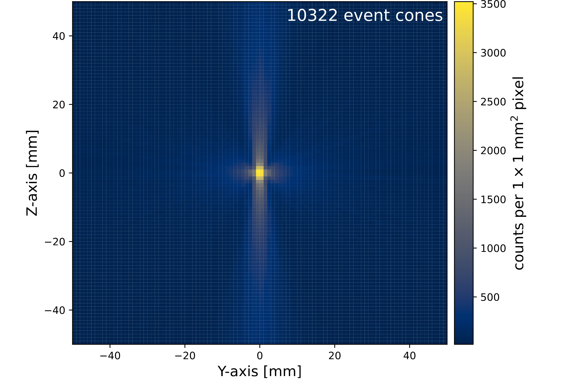
While the elastic scattering line is still very prominent, some new interesting features emerge from inelastic and other nonelastic reactions¹ with carbon. One approach would be to simply filter out these new events by rejecting $\theta$ values which exceed some absolute or fractional difference from the estimated $\theta_\mathrm{est}$. This is not the most future-proof approach for the aforementioned reasons, but it is simple and quite effective, as illustrated for a 5% fractional difference threshold in Figure 6.

Figure 6. Same as Figure 5 but eliminating all events whose calculated θ closest to θ_est deviates by more than 5% from it. Of these 10322 event cones, 7501 were attributed to proton recoils and 2821 to carbon recoils.

This approach / last step is more for illustration and should NOT used experimentally as it also “forces the right answer”, i.e., we only image the cones that yield the image we’re expecting. In experimental work, the fairer angular constraint to place on the cones is that they be pointing in the general $2\pi$ direction toward the source. Thus, the net effect of including all of these nonelastic scattering events is added noise/blurring in the neutron images.

It may be possible that nonelastic events can be considered in some more clever way, rather than just being a source of noise, but this seems unlikely to be feasible experimentally, as the experimental data is not remotely as clean as the MC truth data presented here, making it seemingly impossible to distinguish elastic and nonelastic interactions in any practical and fair way. Still, with good pulse shape discrimination, it may be possible to reliably distinguish proton from carbon recoils as well as the alphas from carbon breakup reactions.

Gamma-ray cone generation

The primary challenge in generating event cones for gamma rays is event sequencing. Owing to the tight bar spacing in NOVO, time resolution of the measurement apparatus, and light-speed velocity of gamma rays, the experimentally produced timestamps for gamma rays are effectively meaningless for determining the actual order of the three coincident interactions. Thus, some other approach must be developed for determining the true, or at least most probable, sequencing of the three interactions.

Fortunately, there are only six possible arrangements for three interactions (123, 132, 213, 231, 312, and 321), and all combinations can be tested. When solving Equation (15) for $\theta_1$, the kinematically nonsensical arrangements will make themselves evident by yielding a value outside of $[-1,1]$ for the argument of $\arccos$ or returning a $\theta_1$ of 0. Eliminating these leaves only the potentially valid sequences of the three interactions. Plotting all these calculated $\theta$ values against the Monte Carlo true $\theta$ for the simulation of a 2 MeV gamma-ray source described earlier yields Figure 7.

Figure 7. Comparison of calculated and MC truth gamma-ray scattering angles θ for all valid gamma-ray event cones in each event

Here, a clear line is present consisting of the correctly calculated $\theta$ values, but they are in a sea of faulty cones. While one could image all of these cones, it would be more computationally expensive and produce a noisier image. The next logical step would be, rather than selecting all potentially valid cones for each event, to select the “best” cone among the valid ones for each event. At present, in a similar fashion to the neutron cone generation, all valid cone angles are compared to the angle $\theta_\mathrm{est}$ between $\hat{D}$ and the vector from the cone vertex $O$ to the estimated source location, and whichever is closest is picked as the “best” cone. This is shown in Figure 8.

Figure 8. Same as Figure 7 but only selecting for each event the “best” cone whose θ is closest to the estimated angle θ_est between the direction vector and the vector from the vertex to source location.

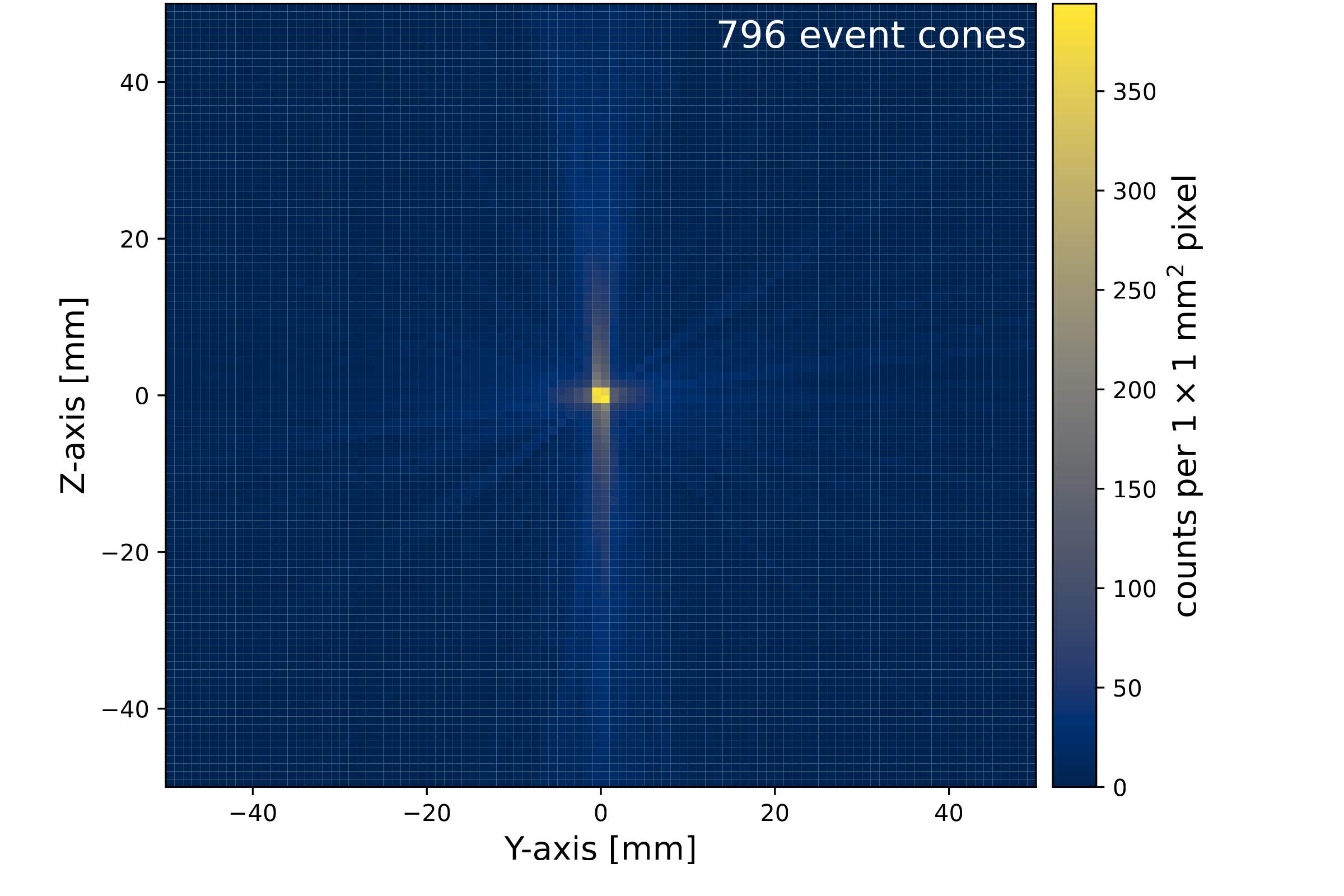
This eliminates almost all errant $\theta$ values. Given that the remaining calculated $\theta$ deviating from the Monte Carlo true $\theta$ are already the “best” of the possible valid $\theta$, it makes sense to conclude that these events correspond to situations where the earlier assumptions (that all interactions are Compton scattering and that all recoil electrons stop in the bars) prove to be false. This, however, is only a very tiny minority of events. Similar to the neutron cone generation method, an arbitrary maximum deviation from an estimated $\theta_\mathrm{est}$ can be enforced and is illustrated for a 5% fractional difference threshold in Figure 9. (Again, this final cleaning step should NOT done for experimental data.)

Figure 9. Same as Figure 8 but eliminating all events whose calculated θ closest to θ_est deviates by more than 5% from it.

With this approach, accurate event cones can be constructed for nearly all gamma-ray events. However, other approaches for selecting the “best” cones may need to be considered in the future depending on the magnitude of measurement uncertainties.

Imaging

What I am calling “imaging” is the process of projecting a constructed event cone—with a vertex coordinate $O=(x_O,y_O,z_O)$, axis/direction unit (column) vector $\hat{D}=\langle u,v,w \rangle^\intercal$, and interior half-angle $\theta$—onto a two-dimensional plane to create an image. Mathematically, this cone is described as the set of all points $X = [x_X,y_X,z_X]^\intercal$ which satisfy [5]:

\begin{equation} (X-O)^\intercal M (X-O) = 0 \label{eq:cone} \end{equation}

Where:

\begin{equation} M = \hat{D}\hat{D}^\intercal - \cos^2(\theta)I_{3\times3} \label{eq:cone_M} \end{equation}

For simplicity, let:

\begin{gather} U = X - O = \begin{bmatrix} x_X - x_O \\ y_X - y_O \\ z_X - z_O \end{bmatrix} = \begin{bmatrix} x_U \\ y_U \\ z_U \end{bmatrix} \label{eq:simplify} \end{gather}

And substitute \ref{eq:simplify} into \ref{eq:cone} and expand:

\begin{gather} \begin{bmatrix} x_U & y_U & z_U \end{bmatrix} \begin{bmatrix} M_{00} & M_{01} & M_{02} \\ M_{10} & M_{11} & M_{12} \\ M_{20} & M_{21} & M_{22} \end{bmatrix} \begin{bmatrix} x_U \\ y_U \\ z_U \end{bmatrix} = 0 \label{eq:cone_matrix} \end{gather}

Multiplying the matrices gives us a second-order polynomial describing the cone:

\begin{align} x_U^2M_{00} + y_U^2M_{11} + z_U^2M_{22} + x_Uy_U(M_{01}+M_{10}) \notag\\ {} + y_Uz_U(M_{12}+M_{21}) + x_Uz_U(M_{02}+M_{20}) &= 0 \label{eq:cone_poly} \end{align}

The mathematics is simpler if forcing the imaging plane to be perpendicular to a coordinate axis. While the ng-imager implementation allows arbitrary plane orientations, the same underlying mathematics applies after expressing coordinates in the plane’s basis, which is assumed for the sake of simplifying this discussion. The image generation process is as follows:

1. Define an imaging plane/window with two points, $P_{BL}$ and $P_{TR}$, denoting the bottom-left and top-right corners of the imaging window, which have one matching coordinate variable whose axis the plane lies perpendicular to. This will set the corresponding element of $X$ to a constant.

2. Define the horizontal and vertical spatial pixel resolutions (e.g., 1 mm). Extract from $P_{BL}$ and $P_{TR}$ the horizontal and vertical bounds of the imaging window. Create 1D arrays for the bin centers and bin edges for both the columns and rows of the image, and create a 2D array $G$ of zeros corresponding to the image rows and columns (referred to as the image array).

3. For each cone:

   1. Initialize two empty lists for storing horizontal and vertical coordinates, $L_H$ and $L_V$, respectively.

   2. Loop through the horizontal bins and in each:

      1. Set the corresponding element of $X$ to the bin center.

      2. Calculate the two known elements of $U$ provided $X$.

      3. Solve Equation (20) for the remaining unknown element of $U$.

      4. Substitute the real $\mathbb{R}$ root(s) found into Equation (18) to obtain the value(s) of last unknown element of $X$.

      5. Append the found value(s) for the $X$ elements corresponding to the image’s horizontal and vertical axes to their respective lists $L_H$ and $L_V$.

   3. Repeat the same loop as above but for the vertical bins.

   4. Score/tally the coordinate pairs in $L_H$ and $L_V$ in a 2D histogram of the same dimensions as the 2D image array $G$ defined earlier and using the bin edges defined earlier. Set all nonzero entries in the histogram to 1.

   5. Add the histogram to the 2D image array $G$.

4. Plot the 2D image array $G$ to show the obtained image.

There are a few notes to be made about this approach. First, the image window is “scanned” in both the horizontal and vertical directions to ensure that each ellipse (technically, conic section, but usually an ellipse) in the imaging window is “continuous” from pixel to pixel. Additionally, the current method is only counting pixels as hit or not hit. Rather than this binary approach, a fancier approach could incorporate the length of the ellipse segment within each pixel and weight them accordingly but is not explored here.

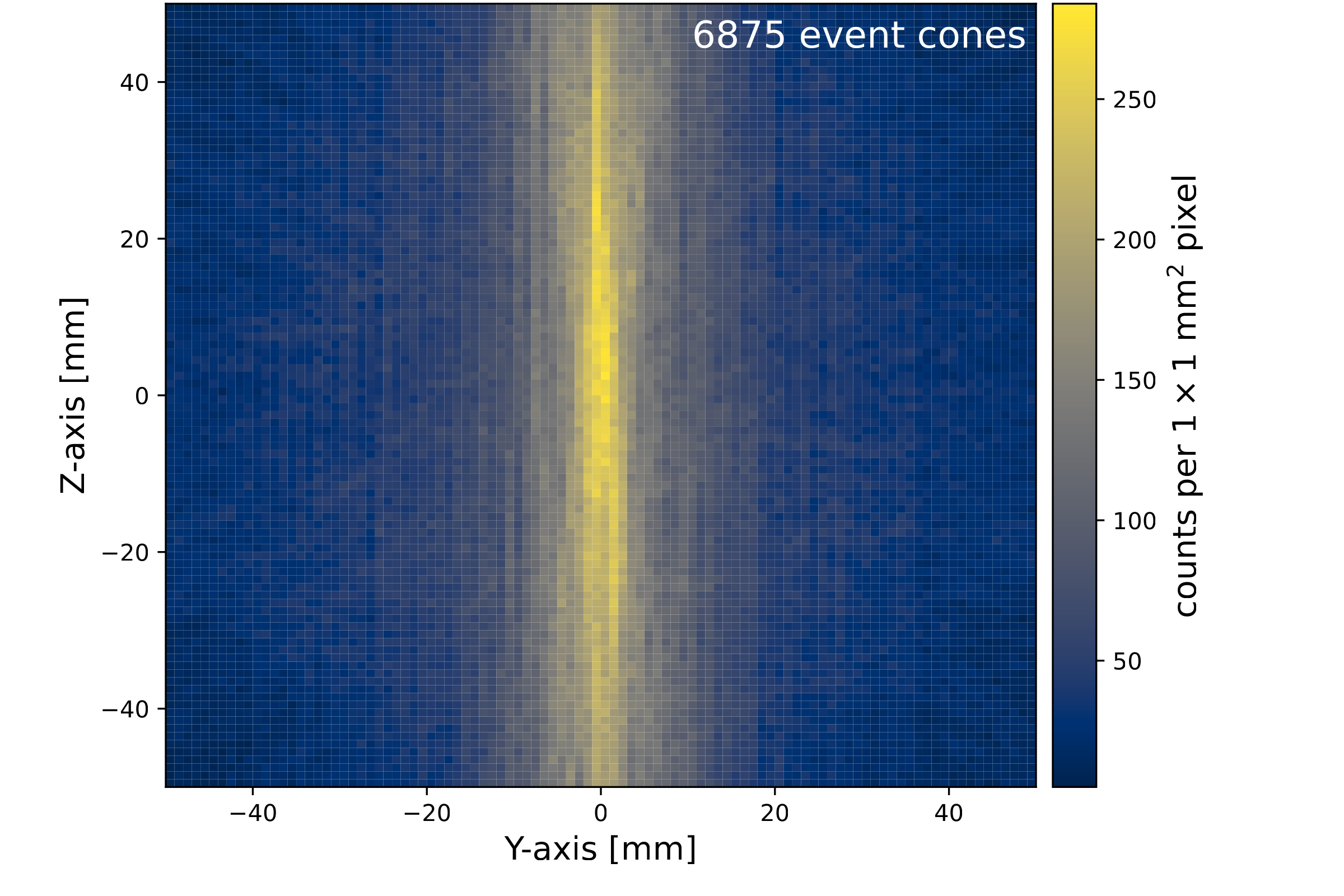
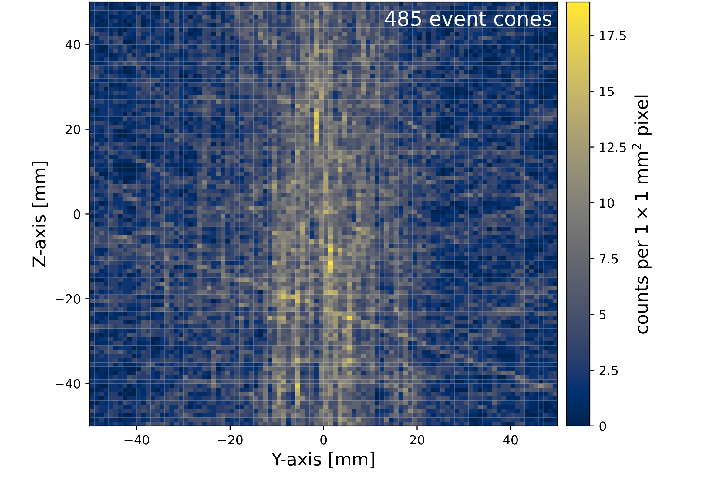
Using this method, Figure 10a is generated for a 1 mm$^2$ pixel resolution and 100 mm wide and tall image window centered on the source location (0,0,0), using the neutron event cones generated earlier, employing results from all nuclear reactions but filtering out rejected events (see Figures 5 vs. 6 earlier). The same image but for the gamma-ray event cones generated earlier (see Figure 9) is shown in Figure 10b.

(a) 14.1 MeV neutron image

(b) 2 MeV gamma-ray image

Figure 10. The images generated from neutron and gamma-ray events simulated earlier.

As a bit of a fun simulation and to test a non-trivial source, next was simulated and imaged a ring-shaped source centered at (0,30,40) with inner radius 48 mm and outer radius 52 mm, isotropically emitting 14.1 MeV neutrons. Its image is shown in Figure 11 and verifies the imaging approach is working as intended.

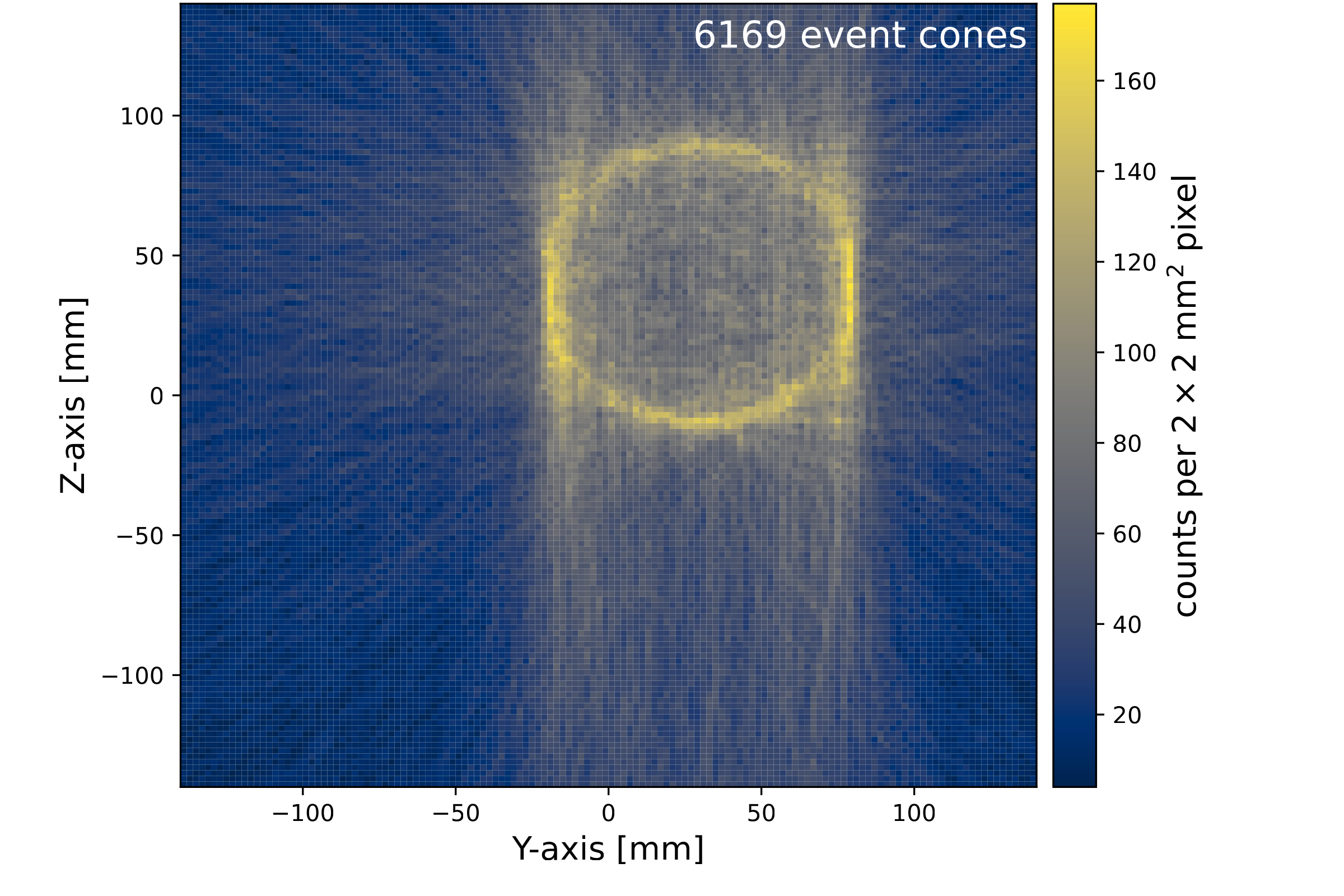
Figure 11. Image of a neutron ring-shaped source.

Effect of using “realistic” interaction coordinates

In the images thus far, all interaction coordinates have used the exact MC true values. In the real experiment, we must assume that every interaction happens at the center of the bar in two dimensions and only has granularity along the depth of interaction (DOI) axis. Figure 12 shows the exact same image as earlier with Figure 10 but only using the exact MC coordinate for the DOI axis and using the location of the bar’s centerline for the other two dimensions, keeping everything else unchanged.

(a) 14.1 MeV neutron image

(b) 2 MeV gamma-ray image

Figure 12. Same as Figure 10 but using the bar centerline coordinates for each interaction position for two of the coordinate axis values and the MC true value along the DOI axis.

To make matters worse, experimental position resolution / uncertainties in the DOI axis actually tend to be worse / greater than those in the bar’s two cross sectional directions. Fortunately though, with enough statistics these issues can, at least to some degree, be overcome.

Conclusions

A consistent methodology for constructing, selecting, and filtering event cones for both neutrons and gamma rays has been outlined here. Provided “pure” Monte Carlo data, the methods perform very well. The analytic, raster scanning-esque implementation of simple back projection employed here performed very well, producing consistently high-quality images.

References

[1] T. Sato, Y. Iwamoto, S. Hashimoto, T. Ogawa, T. Furuta, S. Abe, T. Kai, P.-E. Tsai, N. Matsuda, H. Iwase, N. Shigyo, L. Sihver, and K. Niita, “Features of Particle and Heavy Ion Transport code System (PHITS) version 3.02,” Journal of Nuclear Science and Technology, vol. 55, no. 6, pp. 684-690, 2018. doi: 10.1080/00223131.2017.1419890

[2] R. Fitzpatrick, Newtonian Dynamics. The University of Texas at Austin (online), 2008.

[3] J. A. Bernard, 22.05 Neutron Science and Reactor Physics, Fall 2006 (online), 2006.

[4] I. Meric, E. Alagoz, L. B. Hysing, T. Kögler, D. Lathouwers, W. R. B. Lionheart, J. Mattingly, J. Obhodas, G. Pausch, H. E. S. Pettersen, H. N. Ratliff, M. Rovituso, S. M. Schellhammer, L. M. Setterdahl, K. Skjerdal, E. Sterpin, D. Sudac, J. A. Turko, and K. S. Ytre-Hauge, “A hybrid multi-particle approach to range assessment-based treatment verification in particle therapy,” Scientific Reports, vol. 13, no. 1, p. 6709, 2023. doi: 10.1038/s41598-023-33777-w

[5] D. Armstrong, “Where is the cone?” arXiv:1708.07093, 2018. arXiv:1708.07093